01: Underactuated Control

We consider the BeaverCube 2 CubeSat being built by the MIT STAR Lab.

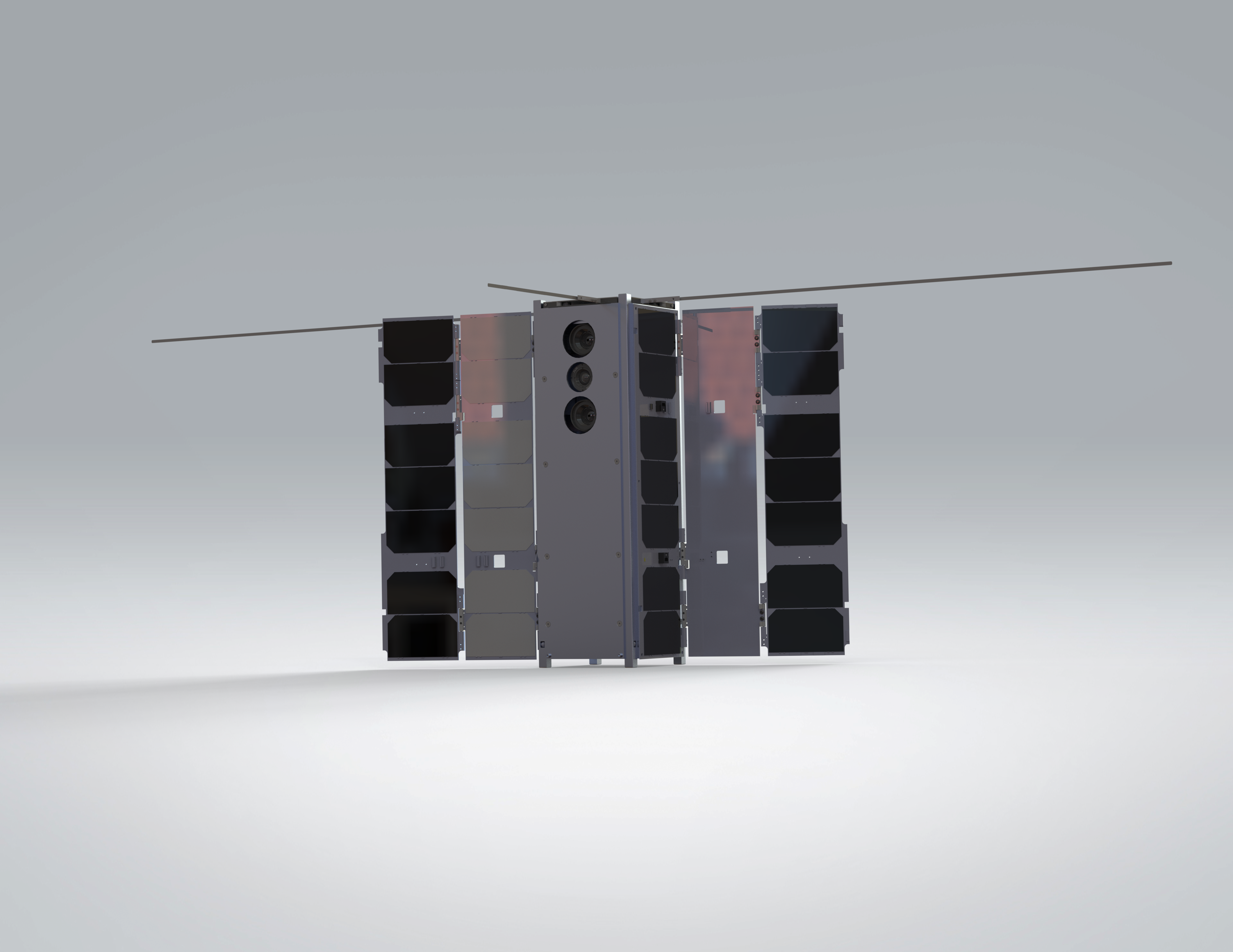
Notably, BeaverCube 2 has a heterogeneous actuator layout of 3 magnetorquers (MTQs) and 1 reaction wheel (RW). We will simulate the CubeSat tracking a ground target using an underactuated control law.

Simulation Configuration

Component	Description
Actuators	Heterogeneous set of 3 Magnetorquers (MTQ) and 1 Reaction Wheel (RW), with parameters matching flight hardware.
Sensors	Set of 3 Magnetometers (MTM).
Satellite	Mass of 4 kg, Inertia Matrix \(J_0 = diag([0.03, 0.03, 0.01]) kg \cdot m^{2}\).
Initial State	The starting attitude state vector consisting of angular velocity, quaternion orientation, and RW momentum: \([\boldsymbol{\omega}, \mathbf{q}, \mathbf{h}]\).
Controller	An underactuated control law with user-specified proportional, derivative, and coupling gains.
Goal	A specific ground target (Latitude/Longitude) to track.
Orbital State	The initial position and velocity of the spacecraft in orbit.

Following this definition, we simulate the environment and analyze the performance using the built-in animation and plotting functions.

import ADCS as ADCS
import numpy as np
import matplotlib.pyplot as plt

acts = [ADCS.RW(axis=np.array([1, 0, 0]), max_torque=0.0023, J=5.7e-6, h=0.0, h_max=0.0036)]
acts += [ADCS.MTQ(axis, max_torque=0.2) for axis in np.eye(3)]
sens = [ADCS.MTM(axis) for axis in np.eye(3)]

satellite = ADCS.Satellite(mass=4, J_0=np.diag([0.03, 0.03, 0.01]), actuators=acts, sensors=sens, boresight=np.array([0, 0, 1]))
x_0 = np.array([0.01, -0.02, 0.01] + [1, 0, 0, 0] + [0.0])  # w, q, h

controller = ADCS.controller.MTQ_w_RW_LP(est_sat=satellite, p_gain=0.00005, d_gain=0.002, c_gain=0.001, h_target=np.array([0, 0, 0]))

goal = ADCS.goals.Coordinate_Goal(lat=42.36, lon=-71.06, alt=0)
os0 = ADCS.Orbital_State(ephem=ADCS.Ephemeris(),J2000=0.22, R=np.array([5000, 0, 5000]), V=np.array([0, 7.5, 0]))

results = ADCS.simulate(
   x=x_0,
   satellite=satellite,
   controller=controller,
   goal=goal,
   os0=os0,
   dt=1.0,
   tf=500.0
)

ADCS.plot(
   results,
   ADCS.plots.AnimationPlot(goal=goal),
   layout=(1,1),
   title="Underactuated Control Animation",
)

ADCS.plot(
   results,
   ADCS.plots.TargetPlot(),
   ADCS.plots.AngularVelocityPlotCombined(sources=["real"]),
   ADCS.plots.ControlPlotCombined(),
   ADCS.plots.ControlPlotSingle(index=0, title="RW Control Torque"),
   layout=(2,2),
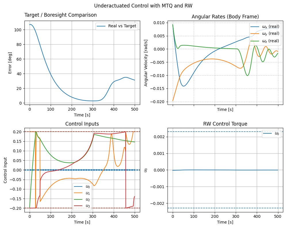
   title="Underactuated Control with MTQ and RW",
)
plt.show()

The results show that the satellite is able to perform a slew despite the underactuated configuration. For most control laws and estimators, we try to make them satellite-agnostic, meaning they should work for most configurations.