04: Complex Estimation
We again consider the TRMM (Tropical Rainfall Measuring Mission) satellite, launched by NASA and JAXA in 1997.
This time, sensors will have biases that must be actively estimated and accounted for.
Component |
Description |
|---|---|
Sensors |
|
Satellite |
Mass of 3000 kg, Inertia Matrix \(J_0 = diag([500, 1500, 1500]) \, kg \cdot m^{2}\). |
Initial State |
The real initial state is set to an angular velocity of \([0.001, 0.001, -0.002] \, rad/s\) and an attitude represented by quaternion \([0.2588, 0, 0.9659, 0]\). |
Estimated Sensors |
|
Estimated Satellite |
Mass of 3200 kg, Inertia Matrix \(J_0 = diag([450, 1400, 1400]) \, kg \cdot m^{2}\). |
Estimated Initial State |
The estimated initial state is set to an angular velocity of \([0, 0, 0] \, rad/s\) and an attitude represented by quaternion \([1, 0, 0, 0]\). |
Estimator |
SRUAKF (Square Root Unscented Kalman Filter) with tuned initial covariance and process noise matrices. |
Orbital State |
The initial position and velocity of the spacecraft in orbit. |
Disturbances |
Include Gravity Gradient disturbance torque on both the real and estimated satellite models. |
import ADCS as ADCS
import numpy as np
from scipy.linalg import block_diag
import matplotlib.pyplot as plt
dt = 20.0
# Real Satellite
gyro_noise = ADCS.Noise(std_noise=3.1623e-7)
gyro_bias = ADCS.Bias(bias=0.1,std_bias=3.1623e-10)
sens = [ADCS.Gyro(axis, noise=gyro_noise, bias=gyro_bias) for axis in np.eye(3)]
mtm_noise = ADCS.Noise(std_noise=50e-9)
mtm_initial_bias = np.array([-0.9948e-9, -0.0199e-9, -0.0995e-9])
for axis, initial_bias in zip(np.eye(3), mtm_initial_bias):
mtm_bias = ADCS.Bias(bias=initial_bias, std_bias=1e-9)
sens += [ADCS.MTM(axis, noise=mtm_noise, bias=mtm_bias)]
sun_noise = ADCS.Noise(std_noise=2e-3)
sun_initial_bias = np.array([0.015, 0.027, -0.009])
for axis, initial_bias in zip(np.eye(3), sun_initial_bias):
sun_bias = ADCS.Bias(bias=initial_bias, std_bias=0.0003)
sens += [ADCS.SunPair(axis, efficiency=0.3,noise=sun_noise, bias=sun_bias)]
gg_dist = [ADCS.disturbances.GG_Disturbance()]
satellite = ADCS.Satellite(mass=3000, J_0=np.diag([500, 1500, 1500]), sensors=sens, disturbances=gg_dist)
x_0 = np.array([0.001, 0.001, -0.002] + [0.2588, 0, 0.9659, 0]) # w, q
# Estimated Satellite
est_gyro_noise = ADCS.Noise(std_noise=3.1623e-7)
est_gyro_bias = ADCS.Bias(bias=0.0,std_bias=3.1623e-10)
est_sens = [ADCS.Gyro(axis, noise=est_gyro_noise, bias=est_gyro_bias, estimate_bias=True) for axis in np.eye(3)]
est_mtm_noise = ADCS.Noise(std_noise=50e-9)
est_mtm_bias = ADCS.Bias(bias=0.0, std_bias=1e-9)
est_sens += [ADCS.MTM(axis, noise=est_mtm_noise, bias=est_mtm_bias, estimate_bias=True) for axis in np.eye(3)]
est_sun_noise = ADCS.Noise(std_noise=2e-3)
est_sun_bias = ADCS.Bias(bias=0.0, std_bias=0.0003)
est_sens += [ADCS.SunPair(axis, efficiency=0.3, noise=est_sun_noise, bias=est_sun_bias, estimate_bias=True) for axis in np.eye(3)]
est_dist_gg = [ADCS.disturbances.GG_Disturbance()]
est_satellite = ADCS.EstimatedSatellite(mass=3000, J_0=np.diag([500, 1500, 1500]), sensors=est_sens, disturbances=est_dist_gg)
x_hat = np.array([0, 0, 0] + [1, 0, 0, 0] + [0, 0, 0] + [0, 0, 0] + [0, 0, 0]) # w, q, gyro_bias, mtm_bias, sun_bias
# Estimator
P_hat = block_diag(
np.eye(3)*(0.01)**2, # Angular Velocity Initial State Error
np.eye(3), # Attitude (MRP) Initial State Error
np.eye(3)*(0.1)**2, # Gyro Initial Bias Error
np.eye(3)*(1e-12)**2,# MTM Initial Bias Error
np.eye(3)*(0.1)**2 # Sun Initial Bias Error
)
sigma_w = 1e-7
Q_w = np.eye(3) * sigma_w * dt
Q_th = np.eye(3) * sigma_w * (dt**3 / 3)
Q_x = np.eye(3) * sigma_w * (dt**2 / 2)
Q_hat = block_diag(
np.block([[Q_w, Q_x],
[Q_x, Q_th]]), # Angular Velocity and Attitude Coupling
np.eye(3) * (1e-10)**2 * dt, # gyro bias RW
np.eye(3) * (1e-9)**2 * dt, # MTM bias RW
np.eye(3) * (1e-4)**2 * dt # Sun bias RW
)
estimator = ADCS.SRUAKF(J2000=0.22, est_sat=est_satellite, x_hat=x_hat, P_hat=P_hat, Q_hat=Q_hat, dt=dt, cross_term=True, quat_as_vec=False)
os0 = ADCS.Orbital_State(ephem=ADCS.Ephemeris(), J2000=0.22, R=np.array([5000, 0, 5000]), V=np.array([0, -7.5, 0]))
results = ADCS.simulate(
x=x_0,
satellite=satellite,
est_satellite=est_satellite,
estimator=estimator,
os0=os0,
dt=dt,
tf=5000.0
)
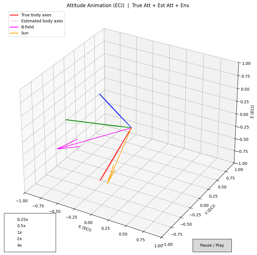
ADCS.plot(
results,
ADCS.plots.AttitudePlot(sources=["real", "estimated"]),
layout=(1,1),
title="Estimator Convergence",
)
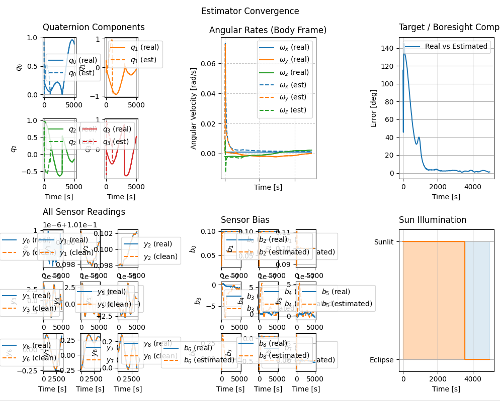
ADCS.plot(
results,
ADCS.plots.QuaternionPlot(sources=["real", "estimated"]),
ADCS.plots.AngularVelocityPlotCombined(sources=["real", "estimated"]),
ADCS.plots.TargetPlot(modes=["real_est"]),
ADCS.plots.SensorsPlot(title="All Sensor Readings", sources=["real", "clean"]),
ADCS.plots.BiasPlot(sources=["real","estimated"]),
ADCS.plots.IlluminationPlot(),
layout=(2,3),
title="Estimator Convergence",
)
plt.show()
Using the correct setup for the \(P\) and \(Q\) matrices, the estimator is able to correctly estimate the biases, and finally converge to the true attitude state. This is despite model mismatches in the satellite and sensors.
|
|
Note that as the satellite enters the eclipse, the estimation quality degrades due to the loss of sun sensor measurements.