03: Simple Estimation¶

All previous examples assumed perfect state knowledge of the satellite. The package provides different estimators to use with various sensors and configurations.

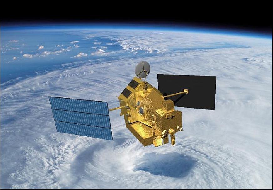
Consider the TRMM (Tropical Rainfall Measuring Mission) satellite, launched by NASA and JAXA in 1997. We will model the satellite with some of its sensors and try to build a simple estimator around it.

Render of the TRMM satellite. (Credit NASA)

Simulation Configuration¶
Component	Description
Sensors	Set of 3 Gyroscopes (Gyro), with noise standard deviation of 0.31623e-7 \(\mu rad/s^{0.5}\). Set of 3 Magnetometers (MTM), with a noise standard deviation of 50 \(nT/s^{0.5}\). Set of 3 Sun Sensors (SunPair), with a noise standard deviation of 2e-3 (unitless) and efficiency of 0.3.
Satellite	Mass of 3000 kg, Inertia Matrix \(J_0 = diag([500, 1500, 1500]) \, kg \cdot m^{2}\).
Initial State	The real initial state is set to an angular velocity of \([0.001, 0.001, -0.002] \, rad/s\) and an attitude represented by quaternion \([0.2588, 0, 0.9659, 0]\).
Estimated Sensors	Set of 3 Gyroscopes (Gyro), with noise standard deviation of 5e-7 \(\mu rad/s^{0.5}\). Set of 3 Magnetometers (MTM), with a noise standard deviation of 50 \(nT/s^{0.5}\). Set of 3 Sun Sensors (SunPair), with a noise standard deviation of 1e-3 (unitless) and efficiency of 0.3.
Estimated Satellite	Mass of 3200 kg, Inertia Matrix \(J_0 = diag([450, 1400, 1400]) \, kg \cdot m^{2}\).
Estimated Initial State	The estimated initial state is set to an angular velocity of \([0, 0, 0] \, rad/s\) and an attitude represented by quaternion \([1, 0, 0, 0]\).
Estimator	SRUAKF (Square Root Unscented Kalman Filter) with tuned initial covariance and process noise matrices.
Orbital State	The initial position and velocity of the spacecraft in orbit.
Disturbances	Include Gravity Gradient disturbance torque on both the real and estimated satellite models.

import os
import sys
sys.path.append(os.path.abspath(os.path.join(__file__, "../../..")))
import ADCS as ADCS
import numpy as np
from scipy.linalg import block_diag
import matplotlib.pyplot as plt

dt = 20.0

# Real Satellite
gyro_noise = ADCS.Noise(std_noise=3.1623e-7)
sens = [ADCS.Gyro(axis, noise=gyro_noise) for axis in np.eye(3)]

mtm_noise = ADCS.Noise(std_noise=5e-8)
sens += [ADCS.MTM(axis, noise=mtm_noise) for axis in np.eye(3)]

sun_noise = ADCS.Noise(std_noise=2e-3)
sens += [ADCS.SunPair(axis, efficiency=0.3,noise=sun_noise) for axis in np.eye(3)]

gg_dist = [ADCS.disturbances.GG_Disturbance()]
satellite = ADCS.Satellite(mass=3000, J_0=np.diag([500, 1500, 1500]), sensors=sens, disturbances=gg_dist)
x_0 = np.array([0.001, 0.001, -0.002] + [0.2588, 0, 0.9659, 0]) # w, q

# Estimated Satellite
est_gyro_noise = ADCS.Noise(std_noise=5e-7)
est_sens = [ADCS.Gyro(axis, noise=est_gyro_noise) for axis in np.eye(3)]

est_mtm_noise = ADCS.Noise(std_noise=5e-8)
est_sens += [ADCS.MTM(axis, noise=est_mtm_noise) for axis in np.eye(3)]

est_sun_noise = ADCS.Noise(std_noise=1e-3)
est_sens += [ADCS.SunPair(axis, efficiency=0.3, noise=est_sun_noise) for axis in np.eye(3)]

est_gg_dist = [ADCS.disturbances.GG_Disturbance()]
est_satellite = ADCS.EstimatedSatellite(mass=3200, J_0=np.diag([450, 1400, 1400]), sensors=est_sens, disturbances=est_gg_dist)
x_hat = np.array([0, 0, 0] + [1, 0, 0, 0]) # w, q

# Estimator
P_hat = block_diag(
    np.eye(3)*(0.01)**2, # Angular Velocity Initial State Error
    np.eye(3), # Attitude (MRP) Initial State Error
    )
Q_hat = block_diag(
    np.eye(3)*(1e-8)**2.0,
    1e-8*np.eye(3)
)
estimator = ADCS.SRUAKF(J2000=0.22, est_sat=est_satellite, x_hat=x_hat, P_hat=P_hat, Q_hat=Q_hat, dt=dt, cross_term=True, quat_as_vec=False)

os0 = ADCS.Orbital_State(ephem=ADCS.Ephemeris(), J2000=0.22, R=np.array([5000, 0, 5000]), V=np.array([0, -7.5, 0]))

results = ADCS.simulate(
    x=x_0,
    satellite=satellite,
    est_satellite=est_satellite,
    estimator=estimator,
    os0=os0,
    dt=dt,
    tf=5000.0
)

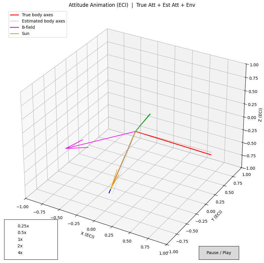
ADCS.plot(
    results,
    ADCS.plots.AttitudePlot(sources=["real", "estimated"]),
    layout=(1,1),
    title="Estimator Convergence",
)

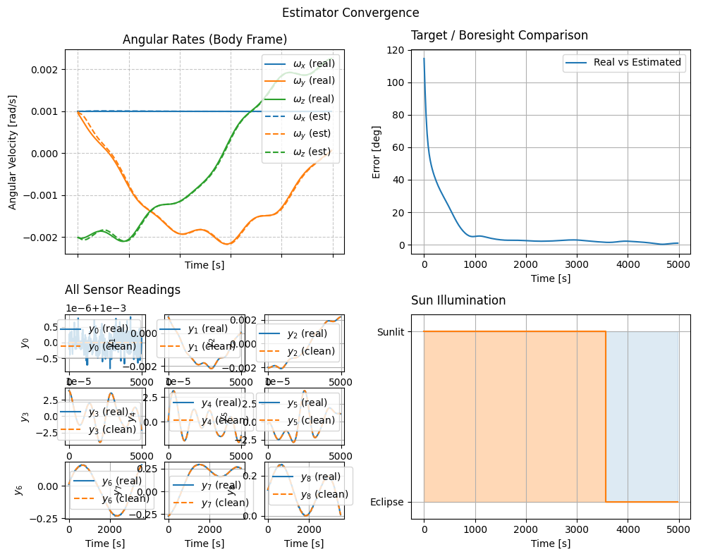
ADCS.plot(
    results,
    ADCS.plots.AngularVelocityPlotCombined(sources=["real", "estimated"]),
    ADCS.plots.TargetPlot(modes=["real_est"]),
    ADCS.plots.SensorsPlot(title="All Sensor Readings", sources=["real", "clean"]),
    ADCS.plots.IlluminationPlot(),
    layout=(2,2),
    title="Estimator Convergence",
)
plt.show()

Note that in the configuration, we may not have perfect knowledge of the satellite’s mass and inertia properties, as well as the sensor characteristics. The estimator is able to converge to the true state over time despite these uncertainties, as shown in the plots below.